Croatia Earthquake on Twitter
There was a strong earthquake on 29. 12. 2020 in Croatia that was felt all over the region. Let’s see how people tweeted about it.
Download the Tweets
library(tidyverse)
library(reshape2)
library(rtweet)
library(scales)
library(lubridate)
We will download the tweets that include the word “earthquake” in
Slovenian, Croatian, Serbian, Bosnian, English, German, Italian or
Hungarian language. I have set the upper limit n to 200.000 because we
want to get as many tweets as possible.
tweets <- search_tweets("potres OR zemljotres OR earthquake OR erdbeben OR terremoto OR földrengés OR foldrenges",
                        n = 200000, retryonratelimit = TRUE, include_rts = FALSE)
This will run for about an hour and will only return data from the past 6-9 days. The final table contains 117.811 tweets.
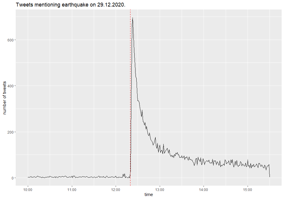
Plot the Time Series
The code below plots the total number of tweets around the earthquake time (denoted by the dashed red line).
# utility function for plotting in CET time
date_format_tz <- function(format = "%H:%M", tz = "CET") {
  function(x) format(x, format, tz = tz)
}

tweets %>%
  filter(created_at >= as.POSIXct("2020-12-29 09:00:00", tz = 'UTC'),
         created_at <= as.POSIXct("2020-12-29 14:30:00", tz = 'UTC')
  ) %>%
  ts_plot(by = 'mins') +
  scale_x_datetime(labels = date_format_tz()) +
  geom_vline(xintercept = as.POSIXct("2020-12-29 12:19:54", tz = 'CET'), linetype = "dashed", color = "red") +
  labs(x = "time",
       y = "number of tweets",
       title = "Tweets mentioning earthquake on 29.12.2020."
       )
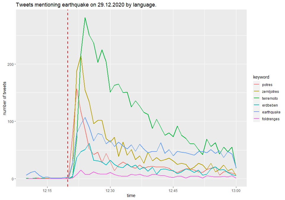
We can also plot the number of tweets by individual earthquake keyword used in the query at the beginning. Every tweet can, in principle, contain the word “earthquake” in different languages. It is therefore better to create indicator variables for each language.
tweets_num_by_time <-
  tweets %>%
  filter(created_at >= as.POSIXct("2020-12-29 11:10:00", tz = 'UTC'),
         created_at <= as.POSIXct("2020-12-29 12:00:00", tz = 'UTC')
  ) %>%
  mutate(
    incl_potres = if_else(str_detect(str_to_lower(text), 'potres'), 1, 0),
    incl_zemljotres = if_else(str_detect(str_to_lower(text), 'zemljotres'), 1, 0),
    incl_terremoto = if_else(str_detect(str_to_lower(text), 'terremoto'), 1, 0),
    incl_erdbeben = if_else(str_detect(str_to_lower(text), 'erdbeben'), 1, 0),
    incl_earthquake = if_else(str_detect(str_to_lower(text), 'earthquake'), 1, 0),
    incl_foldrenges = if_else(str_detect(str_to_lower(text), 'földrengés|foldrenges'), 1, 0)
  ) %>%
  mutate(minute = as.POSIXct(round(created_at, "mins"))) %>%
  group_by(minute) %>%
  summarise(potres = sum(incl_potres),
            zemljotres = sum(incl_zemljotres),
            terremoto = sum(incl_terremoto),
            erdbeben = sum(incl_erdbeben),
            earthquake = sum(incl_earthquake),
            foldrenges = sum(incl_foldrenges)
            )
tweets_num_by_time %>%
  melt(id = "minute") %>%
  rename(keyword = variable) %>%
  ggplot(aes(x = minute, y = value, colour = keyword, group = keyword)) +
  geom_line(size = 0.8) +
  geom_vline(xintercept = as.POSIXct("2020-12-29 12:19:54", tz = 'CET'), linetype = "dashed", color = "red", size = 0.8) +
  scale_x_datetime(labels = date_format_tz()) +
  labs(x = "time",
       y = "number of tweets",
       title = "Tweets mentioning earthquake on 29.12.2020 by language."
       )
Time Differences Between Reactions of Countries
The last chart already gives us an idea about the order of reactions to earthquake by country. Let’s take a more detailed look at this.
First, let’s draw a “scatterplot” of individual tweets by the query
keyword and their time of posting. Each dot represents a tweet and some
vertical jitter has been added to get a better sense about their
distributions. (Very few tweets contain keywords from different
languages. Therefore we won’t make a big mistake if we define user’s
language with the case_when statement.)
tweets %>%
  filter(created_at >= as.POSIXct("2020-12-29 11:10:00", tz = 'UTC'),
         created_at <= as.POSIXct("2020-12-29 11:30:00", tz = 'UTC')
  ) %>%
  mutate(earthquake_keyword = case_when(
    str_detect(str_to_lower(text), 'potres') ~ 'potres (SL/HR)',
    str_detect(str_to_lower(text), 'zemljotres') ~ 'zemljotres (SRB/BIH)',
    str_detect(str_to_lower(text), 'erdbeben') ~ 'erdbeben (DE)',
    str_detect(str_to_lower(text), 'terremoto') ~ 'terremoto (IT)',
    str_detect(str_to_lower(text), 'földrengés|foldrenges') ~ 'földrengés (HU)',
    str_detect(str_to_lower(text), 'earthquake') ~ 'earthquake (EN)',
    TRUE ~ NA_character_
  )) %>%
  filter(!is.na(earthquake_keyword)) %>%
  mutate(earthquake_keyword = fct_relevel(earthquake_keyword, 'földrengés (HU)', 'erdbeben (DE)', 'terremoto (IT)', 'zemljotres (SRB/BIH)', 'potres (SL/HR)', 'earthquake (EN)')) %>%
  ggplot(aes(x = created_at, y = earthquake_keyword)) +
  geom_jitter(height = 0.2, width = 0) +
  geom_vline(xintercept = as.POSIXct("2020-12-29 12:19:54", tz = 'CET'), linetype = "dashed", color = "red", lwd = 1) +
  scale_x_datetime(breaks = 'mins',
                   labels = date_format_tz(),
                   limits = c(as.POSIXct("2020-12-29 12:10:00 CET"),
                              as.POSIXct("2020-12-29 12:30:00 CET"))
                   ) +
  labs(x = "time",
       y = "keyword",
       title = "Tweets mentioning earthquake on 29.12.2020 by language."
       )
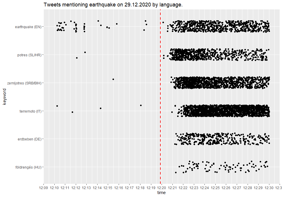
As we can see, the order of countries approximately corresponds to their distance from the epicenter.
Twitter API also returns a column location which can be used to better
identify the user’s country of residence. For most tweets, however, this
column is empty. Some tweets also contain the country or city
information in the text field. Let’s use these columns to draw a
similar chart as above.
tweets %>%
  filter(created_at >= as.POSIXct("2020-12-29 11:10:00", tz = 'UTC'),
         created_at <= as.POSIXct("2020-12-29 11:30:00", tz = 'UTC')
  ) %>%
  mutate(location_clean = case_when(
    str_detect(str_to_lower(paste(location, text)), 'belgrade|beograd|novi sad|serbia') ~ 'Serbia',
    str_detect(str_to_lower(paste(location, text)), 'ljubljana|slovenia|slovenija|maribor') ~ 'Slovenia',
    str_detect(str_to_lower(paste(location, text)), 'zagreb|croatia|hrvatska') ~ 'Croatia',
    str_detect(str_to_lower(paste(location, text)), 'sarajevo|banja luka|bosnia') ~ 'Bosnia and Herzegovina',
    str_detect(str_to_lower(paste(location, text)), 'venezia|veneto|udine|trieste|padova|bologna|treviso|verona|ancona|napoli|milano|milan|roma|italy|italia') ~ 'Italy',
    str_detect(str_to_lower(paste(location, text)), 'wien|vienna|graz|klagenfurt|austria|österreich') ~ 'Austria',
    str_detect(str_to_lower(paste(location, text)), 'budapest|hungary|magyarország') ~ 'Hungary',
    TRUE ~ NA_character_
  )) %>%
  filter(!is.na(location_clean)) %>%
  mutate(location_clean = fct_relevel(location_clean, 'Italy', 'Hungary', 'Austria', 'Serbia', 'Bosnia and Herzegovina', 'Slovenia', 'Croatia')) %>%
  ggplot(aes(x = created_at, y = location_clean)) +
  geom_jitter(height = 0.2, width = 0) +
  geom_vline(xintercept = as.POSIXct("2020-12-29 12:19:54", tz = 'CET'), linetype = "dashed", color = "red", lwd = 1) +
  scale_x_datetime(breaks = 'mins',
                   labels = date_format_tz(),
                   limits = c(as.POSIXct("2020-12-29 12:19:00 CET"),
                              as.POSIXct("2020-12-29 12:30:00 CET"))
                   ) +
  labs(x = "time",
       y = "country",
       title = "Tweets mentioning earthquake on 29.12.2020 by country."
       )
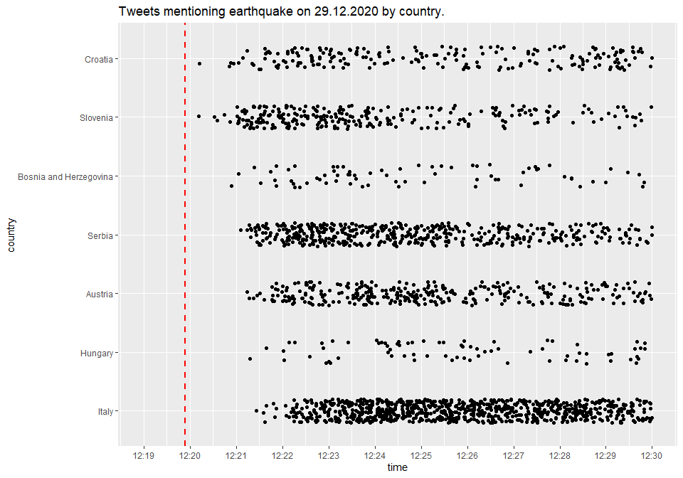
Here the order of countries is a bit different than before. A reason for this is most probably a smaller sample of tweets with location information.
Found this content interesting or useful? Fuel future articles with a coffee!

Session Info
sessionInfo()
## R version 4.0.2 (2020-06-22)
## Platform: x86_64-w64-mingw32/x64 (64-bit)
## Running under: Windows 10 x64 (build 18363)
##
## Matrix products: default
##
## locale:
## [1] LC_COLLATE=Slovenian_Slovenia.1250  LC_CTYPE=Slovenian_Slovenia.1250
## [3] LC_MONETARY=Slovenian_Slovenia.1250 LC_NUMERIC=C
## [5] LC_TIME=Slovenian_Slovenia.1250
##
## attached base packages:
## [1] stats     graphics  grDevices utils     datasets  methods   base
##
## other attached packages:
##  [1] lubridate_1.7.9.2 scales_1.1.1      rtweet_0.7.0      reshape2_1.4.4
##  [5] forcats_0.5.0     stringr_1.4.0     dplyr_1.0.2       purrr_0.3.4
##  [9] readr_1.4.0       tidyr_1.1.2       tibble_3.0.4      ggplot2_3.3.2
## [13] tidyverse_1.3.0
##
## loaded via a namespace (and not attached):
##  [1] tidyselect_1.1.0 xfun_0.19        haven_2.3.1      colorspace_2.0-0
##  [5] vctrs_0.3.6      generics_0.1.0   htmltools_0.5.0  yaml_2.2.1
##  [9] rlang_0.4.9      pillar_1.4.7     glue_1.4.2       withr_2.3.0
## [13] DBI_1.1.0        dbplyr_2.0.0     modelr_0.1.8     readxl_1.3.1
## [17] lifecycle_0.2.0  plyr_1.8.6       munsell_0.5.0    gtable_0.3.0
## [21] cellranger_1.1.0 rvest_0.3.6      evaluate_0.14    labeling_0.4.2
## [25] knitr_1.30       fansi_0.4.1      broom_0.7.3      Rcpp_1.0.5
## [29] backports_1.2.0  jsonlite_1.7.2   farver_2.0.3     fs_1.5.0
## [33] hms_0.5.3        digest_0.6.27    stringi_1.5.3    grid_4.0.2
## [37] cli_2.2.0        tools_4.0.2      magrittr_2.0.1   crayon_1.3.4
## [41] pkgconfig_2.0.3  ellipsis_0.3.1   xml2_1.3.2       reprex_0.3.0
## [45] assertthat_0.2.1 rmarkdown_2.6    httr_1.4.2       rstudioapi_0.13
## [49] R6_2.5.0         compiler_4.0.2